Two-Moment Simulation — Mean and Variance
This article looks at how to simulate a series with a normal distribution — i.e. where the higher moments (skew, excess kurtosis) are zero. For simulation with four moments, see Four-Moment Simulation.
In the first part we look at the univariate case (1 dimension); in the second, we see how to incorporate covariance for more than one dimension.
Univariate simulation (1 dimension)
The idea is to simulate a series
X \sim N(\mu , \sigma)
given \mu and \sigma.
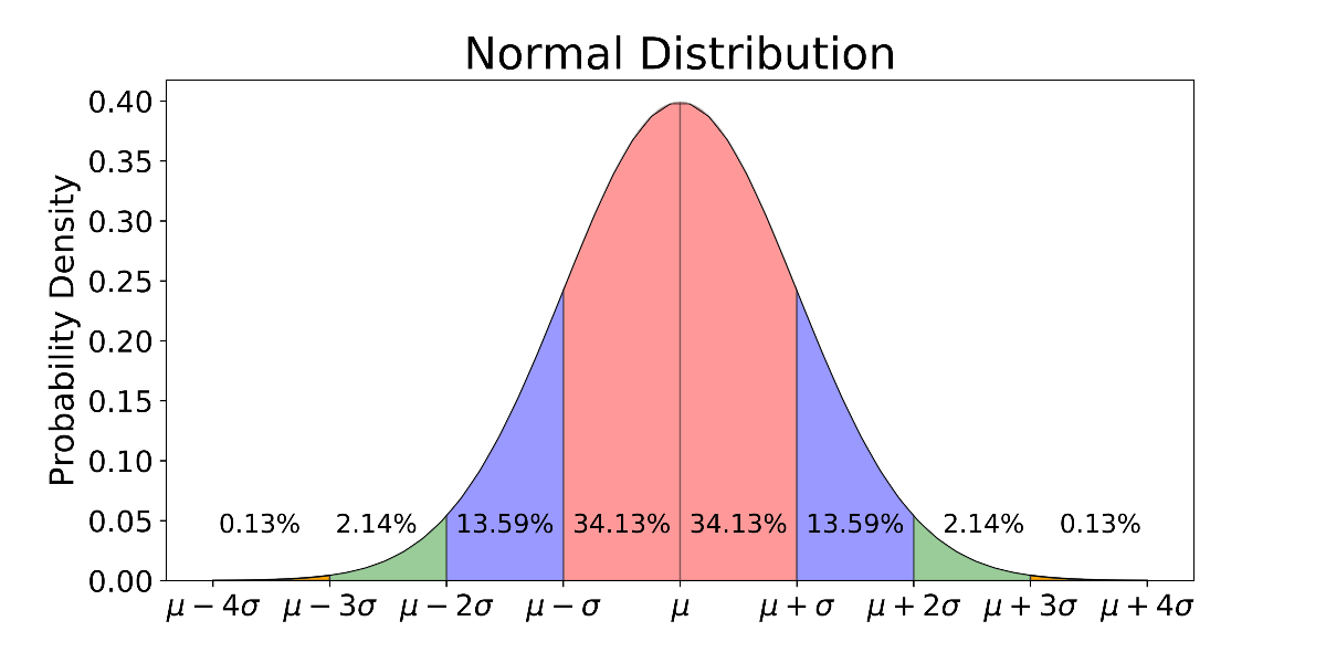
The probability distribution for a random variable that is normally distributed: every point x_i = \mu + z \times \sigma, where z \in (-\infty, \infty).
X \sim N(\mu , \sigma) \mid z \sim N(0,1)
X = \mu + N(0,1) \times \sigma
To generate N(0,1) we can use the Box–Muller transformation. In Excel:
NORM.S.INV(rand())where rand() draws from a uniform distribution on (0,1), and NORM.S.INV is the inverse of the cumulative normal distribution.
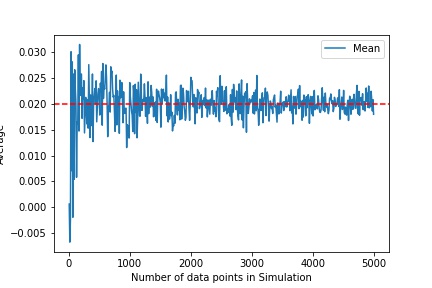
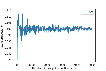
The number of simulated data points is critical to the accuracy of the simulation — more data points lead to higher accuracy.
Higher accuracy for the expected mean and variance with fewer data points can be achieved using random matrix theory — a topic for a future post.
Multivariate simulation (>1 dimension)
The idea is to simulate a series
X \sim N(M , \Sigma)
given M (an array of means) and \Sigma (a covariance matrix).
X = M + N(0,1) \times \sqrt{\Sigma}
where \sqrt{\Sigma} = L is the Cholesky decomposition of \Sigma = LL^T.