Four-Moment Simulation — Mean, Variance, Skew, Kurtosis

Simulate non-normal data points using Fleishman’s power method, targeting all four moments.

In the previous article, Two-Moment Simulation, we discussed how to simulate normally-distributed points for a given mean and standard deviation / covariance matrix.

Here, we discuss how to generate non-normal numbers with a unimodal distribution — i.e. simulate using all four moments (mean, standard deviation, skewness, and kurtosis), ignoring coskewness and cokurtosis.

We refer to the paper by Hao Luo ¹, which uses Fleishman’s power method ² to simulate non-normal data.

The idea is to first simulate a series Y using the power method:

Y \sim D(0,1, \gamma_{1}, \gamma_{2})

where \gamma_1, \gamma_2 are the skewness and excess kurtosis of the distribution D, respectively.

Second, we use our understanding from the previous article to convert the first two moments of D from [0,1] to [\mu, \sigma / \Sigma].

Algorithm

As per the power method, Y can be defined as a third-degree polynomial of X:

Y = a + bX + cX^{2} + dX^{3}

where X \sim N(0,1).

We solve for:

E(Y) = 0,\quad E(Y^{2}) = 1,\quad E(Y^{3}) = \gamma_{1},\quad E(Y^{4}) = \gamma_{2} + 3

The following four equations follow from solving the above:

F_1(b,c,d) : b^2+6bd+ 2c^2 +15d^2-1 =0

F_2(b,c,d) : 2c(b^2+24bd+105d^2+2)-\gamma_1=0

F_3(b,c,d) : 24\big(bd + c^2[1 + b^2 + 28bd] + d^2[12 + 48bd + 141c^2 + 225d^2]\big)-\gamma_2 = 0

a = -c

To solve for a, b, c, d:

\min_{b,c,d} F(b,c,d) = F_1^2(b,c,d)+F_2^2(b,c,d)+F_3^2(b,c,d)

constrained on

F_i(b,c,d) =0 \quad \forall\ i \in (1,3)

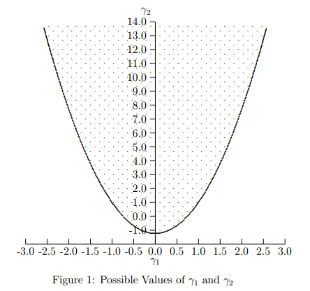
A solution to the above exists only when

\gamma_2 = -1.2264489 + 1.6410373\, \gamma_1^2

Finally, apply the transformation:

Y[\mu, \Sigma, \gamma_1, \gamma_2] = \mu + \sqrt{\Sigma} \times Y[0, 1, \gamma_1, \gamma_2]

Results

Let’s simulate a beta distribution with \alpha = 4.5 and \beta = 1. The left chart shows the PDF of the beta distribution, the simulated beta using the methodology above, and a normal distribution with mean \mu(\text{Beta}(4.5,1)) and standard deviation \sigma(\text{Beta}(4.5,1)). The right chart shows the cumulative distribution of the same, excluding the normal.

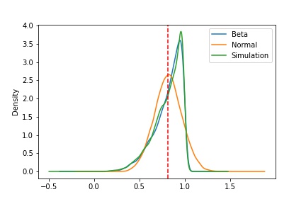
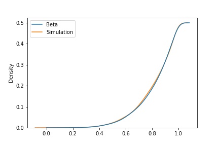
The PDF and its cumulative distribution are very close to each other by the Kolmogorov–Smirnov statistic.

First four moment values for all three cases:

Stat	Beta	Normal	Simulation
Mean	0.82	0.82	0.81
Std	0.15	0.15	0.15
Skew	-1.13	0	-1.08
Kurt	1.02	0	0.88

Footnotes

1. Hao Luo (2011). Generation of Non-normal Data – A Study of Fleishman’s Power Method. diva-portal.org

2. Fleishman, A. I. (1978). A method for simulating non-normal distributions. Psychometrika. springer.com